Introduction
– Variables need to be dimensioned before use. such variables will in memory until the command “exit” or “quit” is entered.
– Command “who“, will list the variables currently in workspace.
– Program lines beginning with “%” are comments.
– If the last character of a statement is a semicolon “;” the command is still executed, but the result is not displayed.
– Creating a vector : a = [ 1 34 2.3 7 3 ]
– Entering a long statement that will not fit on one line : three or more … followed by the carriage return
example : x = 1.234 + 2.345 + 3.456 + 5.678 + 6.678 …
+ 8.789;
– Entering several statements on one line : plot(x,y’,o’),text(1,20,’system1′),text(1,15,’system2)
– when ‘exit’ or ‘quit’ is typed, all variables in MATLAB are lost. if the command ‘save‘ is type befor exiting,
then all variables can be kept in a disk file named matlab.mat. the command ‘load’ will restore the workspace.
– plotting response curve
plot(x,y) (if x and y are vectors of the same lenght)
plot(x1,y1,x2,y2) plotting multiple curves in a single graph
command ‘hold’ can also be used, it freeze the current plot, and inhibits erasure and rescaling.
– adding grid lines, titles of the graph, x-axis label, y-axis label grid (grid lines)
title (graph title)
xlabel ( x-axis label )
ylabel (y-axis label )
– Write a text beginning at point (x,Y)
text(x,y,’sin t’)
plot(x1,y1,x2,y2), text(x1,y1,’1′),text(x2,y2,’2′) mark two curves so they can be distinguished easily
– Product of ploynomials (convolution of the coefficients) a = [ 1 0 -3];b=[ 2 4 5]
c= conv(a,b)
– Division of polynomials
[q,r] = deconv(c,a)
– Polynomial evaluation
if p(s) = 3s^2 + 2s + 1p = [3 2 1]
polyval(p,5)
ans = 86 ( 3*5*5 + 2*5 + 1 = 86)
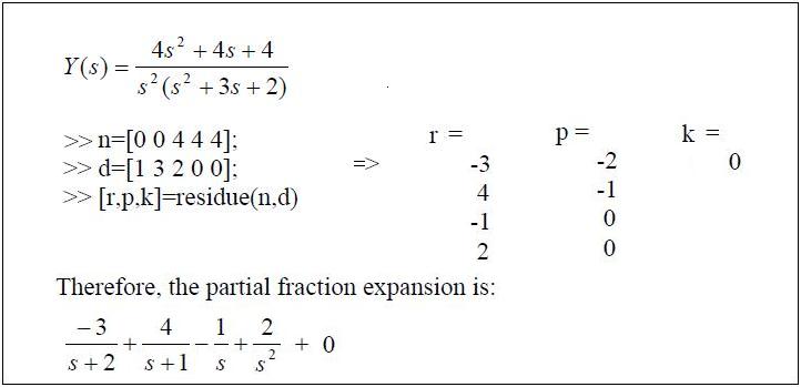
– Partial fraction expansion to perform inverse transform
‘residue’ command
syntax
[r,p,k] = residue(b,a)
[b,a] = residue(r,p,k)
The residue function converts a quotient of polynomials to pole-residue representation, and back again.
.
.
Control
http://www.mathworks.com/help/control/
http://ctms.engin.umich.edu/CTMS/index.php?aux=Extras_step
MATLAB_System_Modeling ( .pdf file)
.
The zeros and poles of H(s)
num = [0 0 4 16 12] ;
den = [1 12 44 48 0] ;
[z, p, K] = tf2zp ( num, den )
.
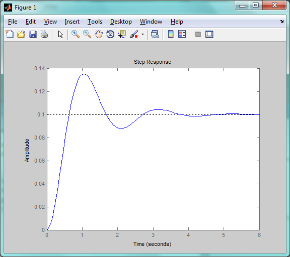
Step Response
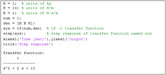
num = 1 ;
den = [1 2 10] ;
sys = tf (num,den)
step (sys) ;
xlabel ( ‘ Time [sec]’ ), ylabel ( ‘Output’ )
title (‘Step response’)
changing the magnitude of the step
step(100*sys)

specifying the time scale
t = 0:0 . 1:10 ;
step (sys,t);
.
.
Impulse response
impulse(sys)
.
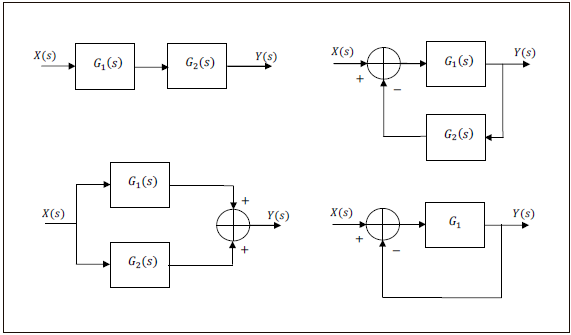
Block Diagrams
[num, den] = series (num1, den1, num2, den2)
[num, den] = parallel (num1, den1, num2, den2)
[num, den] = feedback (num1, den1, num2, den2)
[num, den] = cloop (num1, den1, -1)
printsys (num, den)
example :
num1 = [0 0 10] ;
den1 = [1 2 10] ;
num2 = [0 5] ;
den2 = [1 5] ;
[num, den] = feedback (num1, den1, num2, den2);
printsys (num, den)
num/den =
10 s + 50
————————
s^3 + 7 s^2 + 20 s + 100
.
PID Controller
.
.
.
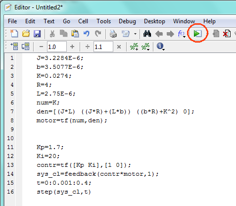
J=3.2284E-6;
b=0;
K=0.0274;
R=4;
L=2.75E-6;
num=K;
den=[(J*L) ((J*R)+(L*b)) ((b*R)+K) 0];
motor=tf(num,den);
Kp=50;
Ki=5000;
contr=tf([Kp Ki],[1 0]);
sys_cl=feedback(contr*motor,1);
t=0:0.001:0.4;
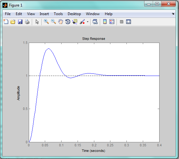
step(sys_cl,t)
.
roots
roots of polynom equation f(x) = 4 x^3 + x + 6
a = [4 0 1 6]
roots(a)
ans =
0.5360 + 1.0545i
0.5360 – 1.0545i
-1.0720
.
Step response
num = [0 0 6.3 18 12.8] ;
den = [1 6 11.3 18 12.8];
step(num,den);
grid;
title(‘unit step ressponse’);
.
.
.
.
.
